Figure 2
Last updated: 2024-12-24
Checks: 5 1
Knit directory: proj_distal/analysis/
This reproducible R Markdown analysis was created with workflowr (version 1.7.1). The Checks tab describes the reproducibility checks that were applied when the results were created. The Past versions tab lists the development history.
Great job! The global environment was empty. Objects defined in the global environment can affect the analysis in your R Markdown file in unknown ways. For reproduciblity it’s best to always run the code in an empty environment.
The command set.seed(12345) was run prior to running the code in the R Markdown file. Setting a seed ensures that any results that rely on randomness, e.g. subsampling or permutations, are reproducible.
Great job! Recording the operating system, R version, and package versions is critical for reproducibility.
Nice! There were no cached chunks for this analysis, so you can be confident that you successfully produced the results during this run.
Great job! Using relative paths to the files within your workflowr project makes it easier to run your code on other machines.
Tracking code development and connecting the code version to the results is critical for reproducibility. To start using Git, open the Terminal and type git init in your project directory.
This project is not being versioned with Git. To obtain the full reproducibility benefits of using workflowr, please see ?wflow_start.
# scRNA-seq
library(Seurat)
#packageVersion("Seurat")

# Plotting
library("ggplot2")
library("ggpubr")
library("cowplot")
library("pheatmap")

# Presentation
library("knitr")

# Others
library("DT")
source(here::here("R/00_generalDeps.R"))
source(here::here("R/output.R"))filt_path <- here::here("data/processed/")Introduction
In this document we are going to perform clustering and plotting figure 2 on the high-quality filtered dataset using Seurat.
Loading umi count and metadata after quality control.
if (file.exists(filt_path)) {
    UMI_df = read.csv(paste0(filt_path,"figure2_input_UMI.csv"), stringsAsFactors = FALSE, header = TRUE, sep=",",check.names=FALSE)
    metadata_df = read.csv(paste0(filt_path,"figure2_input_metadata.csv"), stringsAsFactors = FALSE, header = TRUE, sep=",",check.names=FALSE)
  } else {
    stop("Figure 2 dataset is missing. ",
         "Please check Input first.",
         call. = FALSE)
}
Merge version
Data Preprocessing
Merging Ag reactivity (H1N1 to FLU, PDCE2 TOT to PDCE2)
# adapt nomenclature
metadata_df$Ag_reactivity_v0 = metadata_df$Ag_reactivity
metadata_df$Ag_reactivity = gsub("FLU", "H1N1", metadata_df$Ag_reactivity)
metadata_df$Ag_reactivity = gsub("PDCE2 TOT", "PDCE2", metadata_df$Ag_reactivity)
metadata_df$Ag_reactivity = sapply(metadata_df$Ag_reactivity, function(x) if(x == "C.ALB"){"MP65 (C.ALB)"}
                                   else if(x == "CYP2D6"){"CYP2D6 (LKM1)"}
                                   else if(x == "H1N1"){"MP1 (H1N1)"}
                                   else if(x == "PDCE2"){"PDCE2 (M2)"}
                                   else if(x == "SLA"){"Sepsecs (SLA)"}
                                   else if(x == "SPIKE"){"SPIKE (SARS-CoV-2)"})

df<-metadata_df
df<-df %>%
  group_by(Patient_ID) %>%
  dplyr::count(Ag_reactivity)%>%
  dplyr::mutate(ratio = round(n/sum(n), digit=4))

datatable(df, rownames = T, extensions = 'Buttons',caption="Summary of all dataset cells after motify Ag_reactivity",
          options = list(dom = 'Blfrtip',
                         buttons = c('excel', "csv"),
                         pageLength = 15))
Seurat - Clustering
Setup the Seurat Object
sc_seurat <-CreateSeuratObject(counts = t(UMI_df), min.cells = 1, min.features = 1, project = "huDistal")
#reorder
metadata_df <- metadata_df[colnames(sc_seurat),!colnames(metadata_df) %in% c("nCount_RNA","nFeature_RNA")]
# Add the metadata
for(colname in colnames(metadata_df)){
  sc_seurat@meta.data[,colname]=metadata_df[,colname]
}
Normalizing the data
sc_seurat <- NormalizeData(sc_seurat, normalization.method = "LogNormalize", scale.factor = 10000)feature selection
Based on 4000 highly variable features then filter out TCR gene sets
sc_seurat <- FindVariableFeatures(sc_seurat, selection.method = "vst", nfeatures = 4000)
variable_genes_v = VariableFeatures(sc_seurat)
noTCR_genes_v = variable_genes_v[!grepl("^TR[A,B,D,G][C,V,J]",variable_genes_v)]
VariableFeatures(sc_seurat)=noTCR_genes_v
Scaling the data
Whether to scale the data, False, we’ve center the data, but we don’t scale the expression of each gene.
sc_seurat <- ScaleData(sc_seurat, do.scale = FALSE, verbose = F)The standard workflow for clustering
Dimensional reduction & Cluster the cells & UMAP
sc_seurat <- RunPCA(sc_seurat, verbose = FALSE)
n_pcs = 40
sc_seurat <- RunUMAP(sc_seurat, reduction = "pca", dims = 1:n_pcs, verbose = FALSE)
sc_seurat <- FindNeighbors(sc_seurat, reduction = "pca", dims = 1:n_pcs, verbose = FALSE)

sc_seurat$Ag_reactivity = factor(sc_seurat$Ag_reactivity, levels = c("MP65 (C.ALB)", "CYP2D6 (LKM1)", "MP1 (H1N1)", "PDCE2 (M2)", "Sepsecs (SLA)", "SPIKE (SARS-CoV-2)"))

resolution = 0.8
sc_seurat <- FindClusters(sc_seurat, resolution = resolution, verbose = FALSE)
DimPlot(sc_seurat, group.by = "RNA_snn_res.0.8", label = TRUE) + ggtitle("RNA_snn_res.0.8")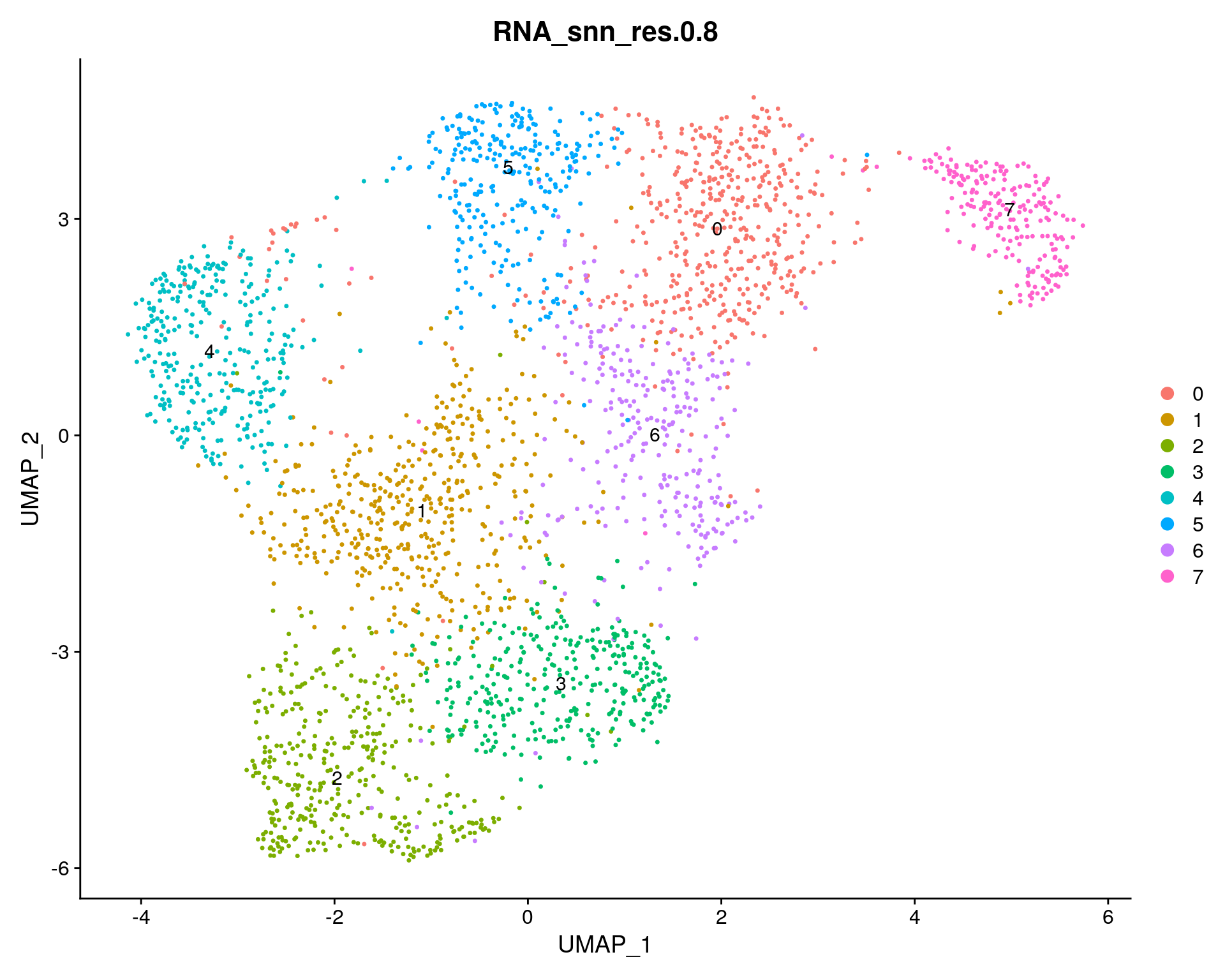
Clusters summary
n_clusts = length(unique(sc_seurat$RNA_snn_res.0.8))

clusterCount = as.data.frame( table( ClusterNumber = sc_seurat[[ "RNA_snn_res.0.8" ]]), responseName = "CellCount");
# Create datatable
datatable( clusterCount,
           class = "compact",
           rownames = FALSE,
           colnames = c("Cluster", "Nb. Cells"),
           options = list(dom = "<'row'rt>", # Set elements for CSS formatting ('<Blf><rt><ip>')
                          autoWidth = FALSE,
                          columnDefs = list( # Center all columns
                            list( targets = 0:(ncol(clusterCount)-1),
                                  className = 'dt-center')),
                          orderClasses = FALSE, # Disable flag for CSS to highlight columns used for ordering (for performance)
                          paging = FALSE, # Disable pagination (show all)
                          processing = TRUE,
                          scrollCollapse = TRUE,
                          scroller = TRUE,  # Only load visible data
                          scrollX = TRUE,
                          scrollY = "525px",
                          stateSave = TRUE));
Finding differentially expressed features
Seurat can help you find markers that define clusters via differential expression (DE)
Idents(object = sc_seurat) <- "RNA_snn_res.0.8"

#parameter
# Parameters for identification of marker annotations for clusters (see Seurat::FindAllMarkers())
FINDMARKERS_METHOD    = "wilcox"  # Method used to identify markers
FINDMARKERS_ONLYPOS   = TRUE;     # Only consider overexpressed annotations for markers ? (if FALSE downregulated genes can also be markers)
FINDMARKERS_MINPCT    = 0.1;      # Only test genes that are detected in a minimum fraction of cells in either of the two populations. Speed up the function by not testing genes that are very infrequently expressed. Default is '0.1'.
FINDMARKERS_LOGFC_THR = 0.25;     # Limit testing to genes which show, on average, at least X-fold difference (log-scale) between the two groups of cells. Default is '0.25'. Increasing logfc.threshold speeds up the function, but can miss weaker signals.
FINDMARKERS_PVAL_THR  = 0.01;    # PValue threshold for identification of significative markers
FINDMARKERS_SHOWTOP   = NULL;       # Number of marker genes to show in report and tables (NULL for all)
# Identify marker genes
markers = FindAllMarkers( object          = sc_seurat,
                          test.use        = FINDMARKERS_METHOD,
                          only.pos        = FINDMARKERS_ONLYPOS,
                          min.pct         = FINDMARKERS_MINPCT,
                          logfc.threshold = FINDMARKERS_LOGFC_THR)

#markers = markers[markers$p_val_adj <= FINDMARKERS_PVAL_THR,]
markers$diff.pct = markers$pct.1 - markers$pct.2

# Filter markers by cluster (TODO: check if downstream code works when no markers found)
topMarkers = by( markers, markers[["cluster"]], function(x)
{
  # Filter markers based on adjusted PValue
  x = x[ x[["p_val_adj"]] < FINDMARKERS_PVAL_THR, , drop = FALSE];
  # Sort by decreasing logFC
  x = x[ order(abs(x[["diff.pct"]]), decreasing = TRUE), , drop = FALSE ]
  # Return top ones
  return( if(is.null( FINDMARKERS_SHOWTOP)) x else head( x, n = FINDMARKERS_SHOWTOP));
});

# Merge marker genes in a single data.frame and render it as datatable
topMarkersDF = do.call( rbind, topMarkers);
# Select and order columns to be shown in datatable
topMarkersDT = topMarkersDF[c("gene", "cluster", "avg_log2FC" , "pct.1", "pct.2","diff.pct", "p_val_adj")]

# Create datatable
datatable( topMarkersDT,
           class = "compact",
           filter="top",
           rownames = FALSE,
           colnames = c("gene", "cluster", "avg_log2FC" , "pct.1", "pct.2","diff.pct", "p_val_adj"),
           caption = paste(ifelse( is.null( FINDMARKERS_SHOWTOP), "All", paste("Top", FINDMARKERS_SHOWTOP)), "marker genes for each cluster"),
           extensions = c('Buttons', 'Select'),
           options = list(dom = "<'row'<'col-sm-8'B><'col-sm-4'f>> <'row'<'col-sm-12'l>> <'row'<'col-sm-12'rt>> <'row'<'col-sm-12'ip>>", # Set elements for CSS formatting ('<Blf><rt><ip>')
                          autoWidth = FALSE,
                          buttons = exportButtonsListDT,
                          columnDefs = list(
                            list( # Center all columns except first one
                              targets = 1:(ncol( topMarkersDT)-1),
                              className = 'dt-center'),
                            list( # Set renderer function for 'float' type columns (LogFC)
                              targets = ncol( topMarkersDT)-2,
                              render = htmlwidgets::JS("function ( data, type, row ) {return type === 'export' ? data : data.toFixed(4);}")),
                            list( # Set renderer function for 'scientific' type columns (PValue)
                              targets = ncol( topMarkersDT)-1,
                              render = htmlwidgets::JS( "function ( data, type, row ) {return type === 'export' ? data : data.toExponential(4);}"))),
                          #fixedColumns = TRUE, # Does not work well with filter on this column
                          #fixedHeader = TRUE, # Does not work well with 'scrollX'
                          lengthMenu = list(c( 10, 50, 100, -1),
                                            c( 10, 50, 100, "All")),
                          orderClasses = FALSE, # Disable flag for CSS to highlight columns used for ordering (for performance)
                          processing = TRUE,
                          #search.regex= TRUE, # Does not work well with 'search.smart'
                          search.smart = TRUE,
                          select = TRUE, # Enable ability to select rows
                          scrollCollapse = TRUE,
                          scroller = TRUE,  # Only load visible data
                          scrollX = TRUE,
                          scrollY = "525px",
                          stateSave = TRUE))
selected clusters
selected antigen reactivity cluster groups of memory CD4 T cells
sc_seurat$Group = sapply(as.numeric(as.character(sc_seurat$RNA_snn_res.0.8)), function(x) if(x == 0 ){"H1N1"}
                          else if(x %in% c(2,3)) {"Auto-reactivity"}
                          else if(x == 5) {"C.ALB"}
                          else if(x == 6){"SARS-CoV-2"}
                          else{x})

clusterCount = as.data.frame( table( ClusterNumber = sc_seurat[[ "Group" ]]), responseName = "CellCount");
# Create datatable
datatable( clusterCount,
           class = "compact",
           rownames = FALSE,
           colnames = c("Cluster", "Nb. Cells"),
           options = list(dom = "<'row'rt>", # Set elements for CSS formatting ('<Blf><rt><ip>')
                          autoWidth = FALSE,
                          columnDefs = list( # Center all columns
                            list( targets = 0:(ncol(clusterCount)-1),
                                  className = 'dt-center')),
                          orderClasses = FALSE, # Disable flag for CSS to highlight columns used for ordering (for performance)
                          paging = FALSE, # Disable pagination (show all)
                          processing = TRUE,
                          scrollCollapse = TRUE,
                          scroller = TRUE,  # Only load visible data
                          scrollX = TRUE,
                          scrollY = "525px",
                          stateSave = TRUE));
metadata_df$Group = sc_seurat$Group
subset = subset(sc_seurat, idents = c(1, 4, 7), invert = TRUE)
DimPlot(subset, reduction = "umap", group.by = "Group", cols = c("C.ALB" = "#F8766D", "H1N1" = "#7CAE00" ,"Auto-reactivity"= "#00BFC4", "SARS-CoV-2"= "#C77CFF")) + ggtitle(paste0("Group: ", length(subset$Group)))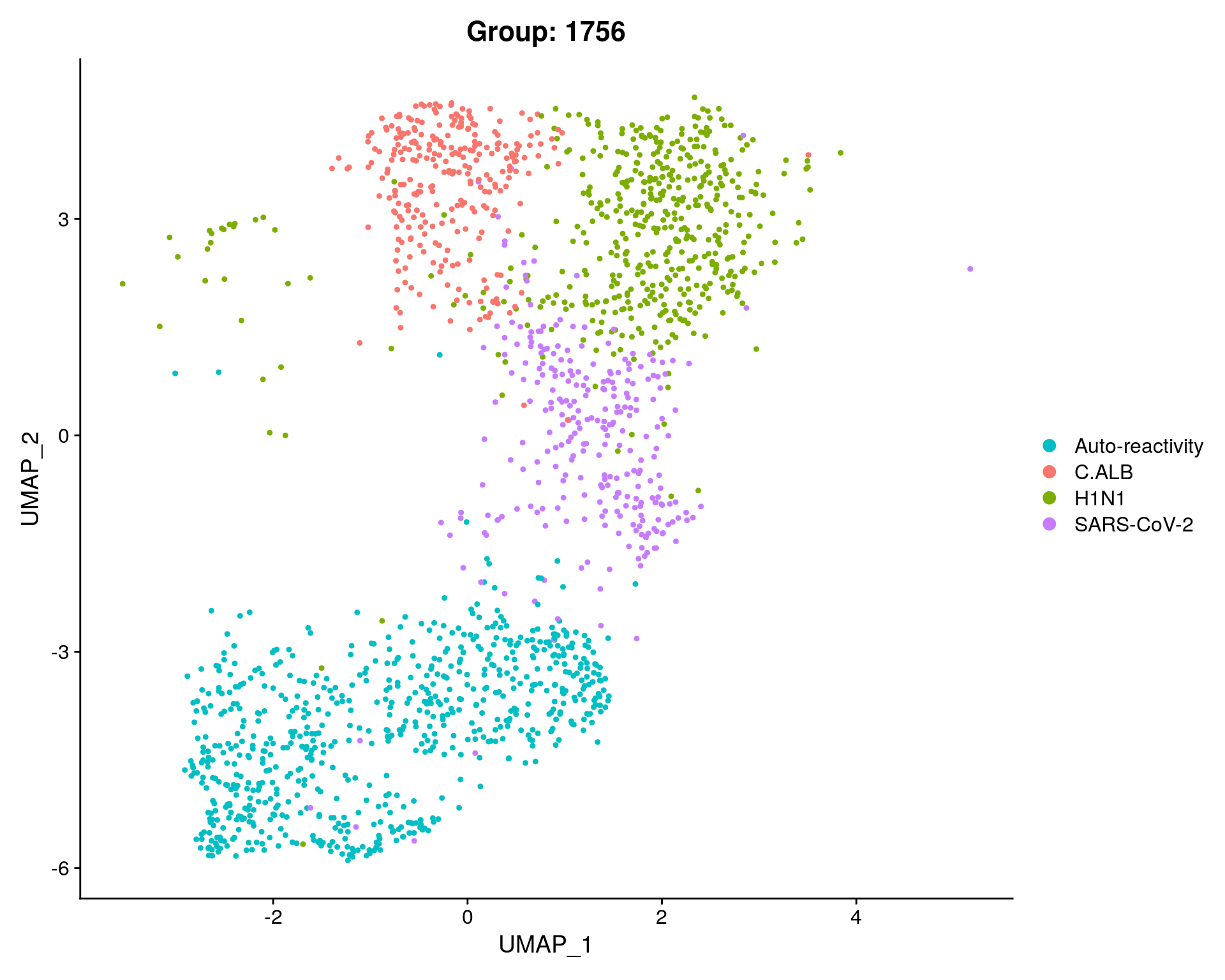
n_clusts_sub = length(unique(subset$Group))

clusterCount = as.data.frame( table( ClusterNumber = subset[[ "Group" ]]), responseName = "CellCount");
# Create datatable
datatable( clusterCount,
           class = "compact",
           rownames = FALSE,
           colnames = c("Group", "Nb. Cells"),
           options = list(dom = "<'row'rt>", # Set elements for CSS formatting ('<Blf><rt><ip>')
                          autoWidth = FALSE,
                          columnDefs = list( # Center all columns
                            list( targets = 0:(ncol(clusterCount)-1),
                                  className = 'dt-center')),
                          orderClasses = FALSE, # Disable flag for CSS to highlight columns used for ordering (for performance)
                          paging = FALSE, # Disable pagination (show all)
                          processing = TRUE,
                          scrollCollapse = TRUE,
                          scroller = TRUE,  # Only load visible data
                          scrollX = TRUE,
                          scrollY = "525px",
                          stateSave = TRUE));
Finding differentially expressed features on cluster groups of memory CD4 T cells
Idents(subset) <- "Group"
# Identify marker genes
markers = FindAllMarkers( object          = subset,
                          test.use        = FINDMARKERS_METHOD,
                          only.pos        = FINDMARKERS_ONLYPOS,
                          min.pct         = FINDMARKERS_MINPCT,
                          logfc.threshold = FINDMARKERS_LOGFC_THR)

#markers = markers[markers$p_val_adj <= FINDMARKERS_PVAL_THR,]
markers$diff.pct = markers$pct.1 - markers$pct.2

# Filter markers by cluster (TODO: check if downstream code works when no markers found)
topMarkers = by( markers, markers[["cluster"]], function(x)
{
  # Filter markers based on adjusted PValue
  x = x[ x[["p_val_adj"]] < FINDMARKERS_PVAL_THR, , drop = FALSE];
  # Sort by decreasing logFC
  x = x[ order(abs(x[["diff.pct"]]), decreasing = TRUE), , drop = FALSE ]
  # Return top ones
  return( if(is.null( FINDMARKERS_SHOWTOP)) x else head( x, n = FINDMARKERS_SHOWTOP));
});

# Merge marker genes in a single data.frame and render it as datatable
topMarkersDF = do.call( rbind, topMarkers);
# Select and order columns to be shown in datatable
topMarkersDT = topMarkersDF[c("gene", "cluster", "avg_log2FC" , "pct.1", "pct.2","diff.pct", "p_val_adj")]

# Create datatable
datatable( topMarkersDT,
           class = "compact",
           filter="top",
           rownames = FALSE,
           colnames = c("gene", "cluster", "avg_log2FC" , "pct.1", "pct.2","diff.pct", "p_val_adj"),
           caption = paste(ifelse( is.null( FINDMARKERS_SHOWTOP), "All", paste("Top", FINDMARKERS_SHOWTOP)), "marker genes for each cluster"),
           extensions = c('Buttons', 'Select'),
           options = list(dom = "<'row'<'col-sm-8'B><'col-sm-4'f>> <'row'<'col-sm-12'l>> <'row'<'col-sm-12'rt>> <'row'<'col-sm-12'ip>>", # Set elements for CSS formatting ('<Blf><rt><ip>')
                          autoWidth = FALSE,
                          buttons = exportButtonsListDT,
                          columnDefs = list(
                            list( # Center all columns except first one
                              targets = 1:(ncol( topMarkersDT)-1),
                              className = 'dt-center'),
                            list( # Set renderer function for 'float' type columns (LogFC)
                              targets = ncol( topMarkersDT)-2,
                              render = htmlwidgets::JS("function ( data, type, row ) {return type === 'export' ? data : data.toFixed(4);}")),
                            list( # Set renderer function for 'scientific' type columns (PValue)
                              targets = ncol( topMarkersDT)-1,
                              render = htmlwidgets::JS( "function ( data, type, row ) {return type === 'export' ? data : data.toExponential(4);}"))),
                          #fixedColumns = TRUE, # Does not work well with filter on this column
                          #fixedHeader = TRUE, # Does not work well with 'scrollX'
                          lengthMenu = list(c( 10, 50, 100, -1),
                                            c( 10, 50, 100, "All")),
                          orderClasses = FALSE, # Disable flag for CSS to highlight columns used for ordering (for performance)
                          processing = TRUE,
                          #search.regex= TRUE, # Does not work well with 'search.smart'
                          search.smart = TRUE,
                          select = TRUE, # Enable ability to select rows
                          scrollCollapse = TRUE,
                          scroller = TRUE,  # Only load visible data
                          scrollX = TRUE,
                          scrollY = "525px",
                          stateSave = TRUE))
Heatmap
norm_df = as.data.frame(t(as.matrix(GetAssayData(subset, slot = "data"))))
heatmap_metadata_df = metadata_df[colnames(subset),]
heatmap_metadata_df$Group =  factor(heatmap_metadata_df$Group, levels= c("C.ALB", "H1N1", "Auto-reactivity", "SARS-CoV-2"))
heatmap_metadata_df<- arrange(heatmap_metadata_df , Group, Patient_ID)

top10 <- topMarkersDT %>% group_by(cluster) %>% top_n(n = 10, wt = diff.pct)
top10$cluster = factor(top10$cluster, levels= c("C.ALB", "H1N1", "Auto-reactivity", "SARS-CoV-2"))
top10<- arrange(top10,cluster)
genes = top10$gene

df= norm_df[heatmap_metadata_df$UniqueCellID,genes]
df <- t(df)

TWO_COLORS_VECTOR=c("#FBE9E7", "#FF3D00")
TWO_COLORS_GRADIANT=c("grey80",colorRampPalette(TWO_COLORS_VECTOR)(n = 2000))

col=c("grey30",TWO_COLORS_GRADIANT[-1])

df= norm_df[heatmap_metadata_df$UniqueCellID,genes]
df <- t(df)

gap.cells =  c(281,  281 +489, 281 +489+710)
gap.genes = c(10,20,30)

annot_colors=list(Ag_reactivity=c("MP65 (C.ALB)"="#F8766D","CYP2D6 (LKM1)"="#B79F00","MP1 (H1N1)"="#00BA38",
                                  "PDCE2 (M2)" ="#00BFC4","Sepsecs (SLA)" = "#619CFF", "SPIKE (SARS-CoV-2)" = "#F564E3"),
                  Patient_ID = c("01-004-08" = "#F8766D",
                                 "01-018-22" = "#E7851E",
                                 "01-028-06" = "#D09400",
                                 "01-140-05" ="#B2A100",
                                 "01-165-03" = "#89AC00",
                                 "01-176-02" = "#45B500",
                                 "01-176-03" ="#00BC51",
                                 "01-188-02" ="#00C087",
                                 "01-192-02" ="#00C0B2",
                                 "01-213-02" ="#00BCD6",
                                 "01-214-02" ="#00B3F2",
                                 "01-232-01" ="#29A3FF",
                                 "01-247-01" ="#9C8DFF",
                                 "05-001-01" ="#D277FF",
                                 "08-003-01" ="#F166E8",
                                 "UKELKM_4"  ="#FF61C7",
                                 "UKELKM_6" ="#FF689E"),
                  Group=c(C.ALB="#F8766D",H1N1="#7CAE00",
                                  "Auto-reactivity" = "#00BFC4", "SARS-CoV-2" = "#C77CFF"))


Annotationcol <-heatmap_metadata_df[,c('Group','Patient_ID','Ag_reactivity')] # dataframe contain
Annotationcol$Group = factor(Annotationcol$Group, levels= c("C.ALB", "H1N1", "Auto-reactivity", "SARS-CoV-2"))

set.seed(123)
pheatmap(df,
         color = col,
         cluster_rows = FALSE,
         cluster_cols = FALSE,
         show_colnames = FALSE,
         show_rownames = TRUE,
         gaps_col = gap.cells,
         gaps_row = gap.genes,
         fontsize_row = 8 ,
         annotation_col = Annotationcol,
         annotation_colors = annot_colors,
         main = "Heatmap order by diff.pct v2")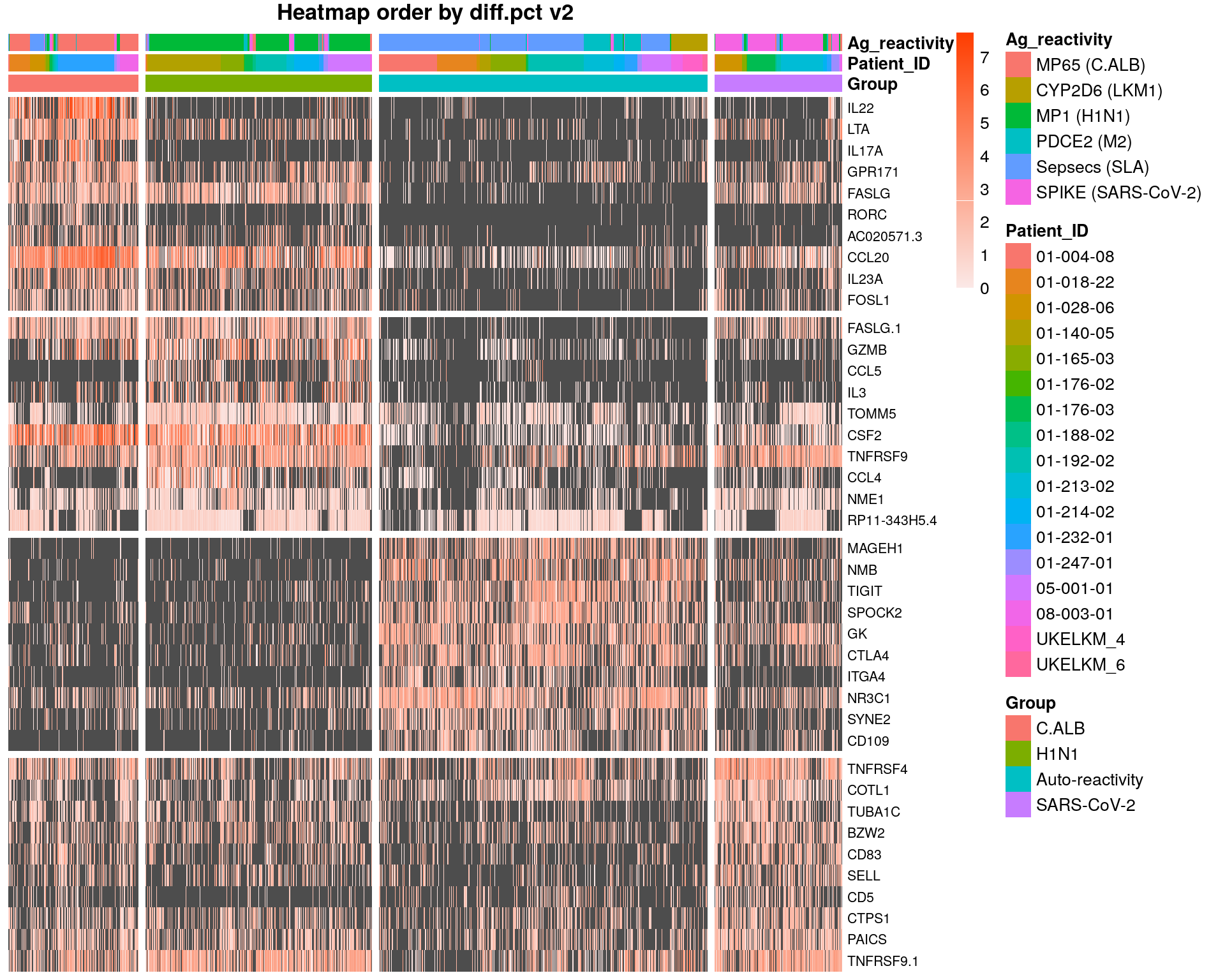
Dotplot
subset$Group = factor(subset$Group, levels= c("C.ALB", "H1N1", "Auto-reactivity", "SARS-CoV-2"))
Idents(subset) <- "Group"

markers = c(
  "CCL20", "IL23A", "IL17A", "IL22",
  "CCL4", "CCL5", "GZMB", "FASLG",
  "CXCL13", "TOX", "CTLA4", "TIGIT",
  "IL4", "IL13", "CCR4", "TNFRSF4")

DotPlot(subset, features = markers) +
  geom_point(aes(size=pct.exp), shape = 21, colour="black", stroke=0.5) +
  scale_colour_gradient2(low = "grey30",  high = "#FD6839") + # color scale
  guides(size=guide_legend(override.aes=list(shape=21, colour="black", fill="white"))) +
  theme(axis.text.x = element_text(angle = 45, hjust=1))  + coord_flip()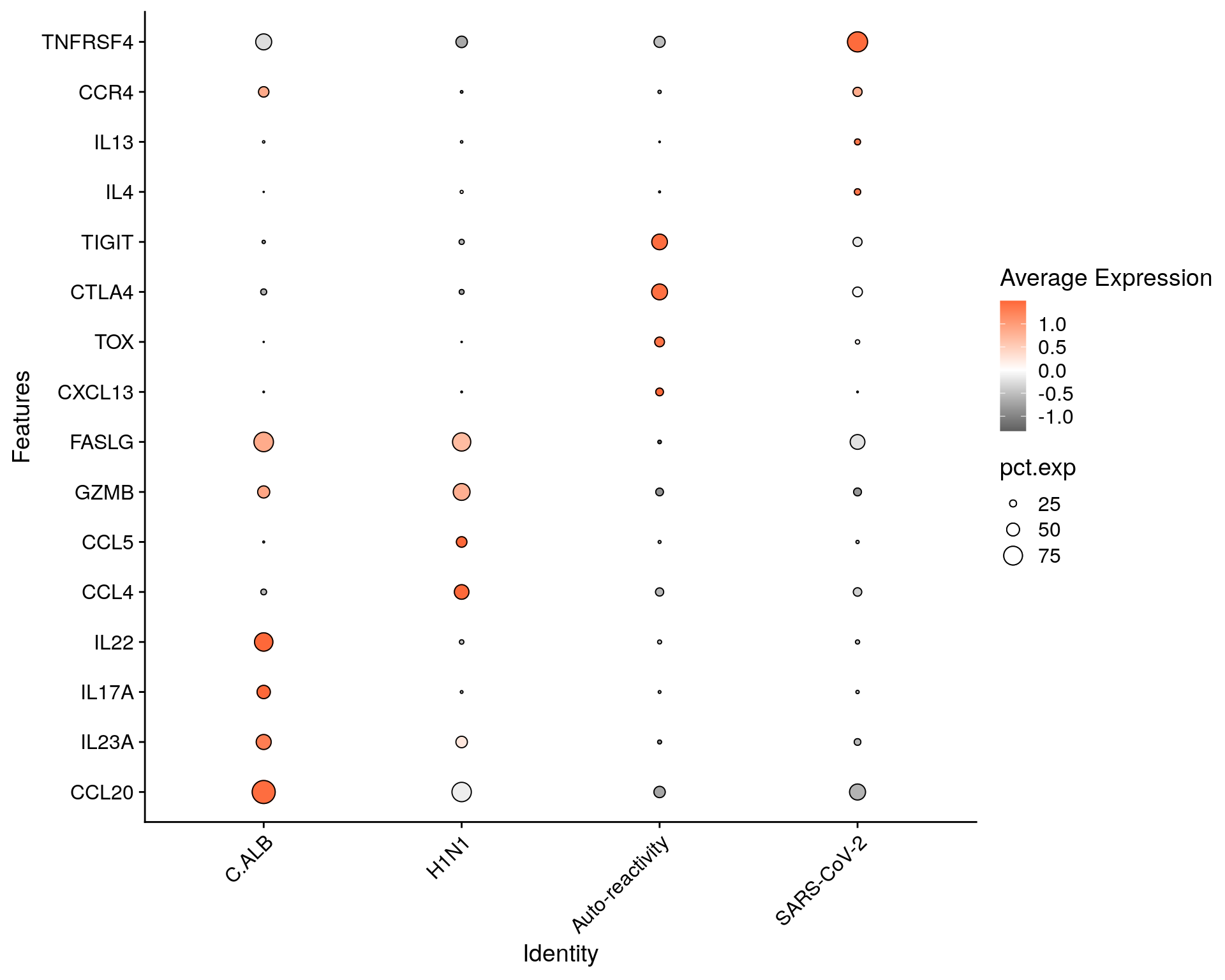
Figure 2
Panel A
fig <- DimPlot(sc_seurat, reduction = "umap", group.by = "RNA_snn_res.0.8", label = T) + ggtitle(paste0("RNA_snn_res.0.8: ", length(sc_seurat$RNA_snn_res.0.8)))

ggsave(here::here("output", DOCNAME, "figure2-panelA.pdf"), fig,
        width = 8, height = 8, scale = 1.2)
ggsave(here::here("output", DOCNAME, "figure2-panelA.png"), fig,
        width = 8, height = 8, scale = 1.2)

fig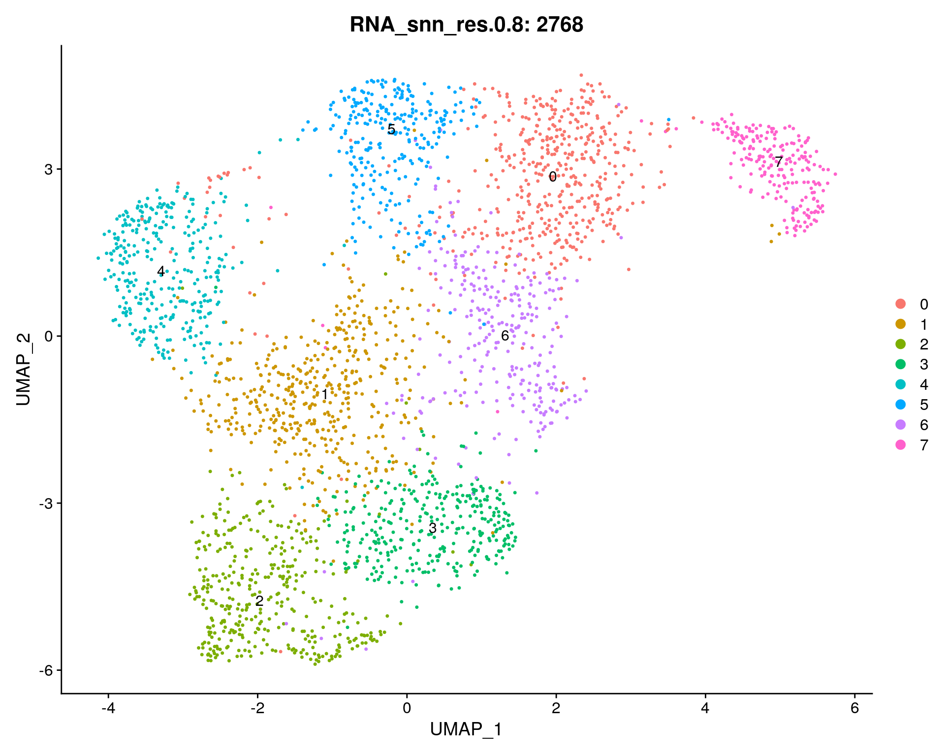
Panel B
fig <- DimPlot(sc_seurat, reduction = "umap", group.by = "Ag_reactivity") + ggtitle(paste0("Ag_reactivity: ", length(sc_seurat$Ag_reactivity)))

ggsave(here::here("output", DOCNAME, "figure2-panelB.pdf"), fig,
        width = 8, height = 8, scale = 1.2)
ggsave(here::here("output", DOCNAME, "figure2-panelB.png"), fig,
        width = 8, height = 8, scale = 1.2)

fig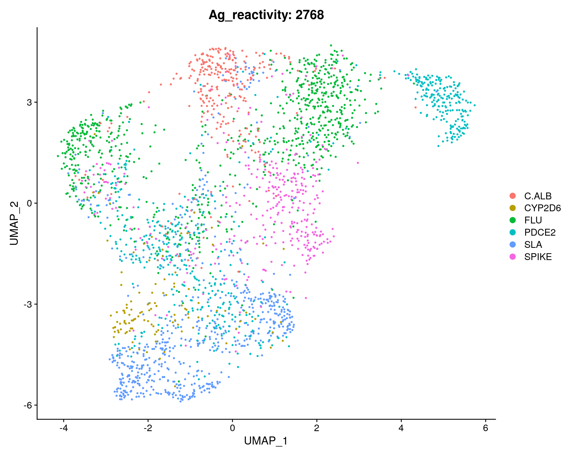
Panel C
fig <- DimPlot(sc_seurat, reduction = "umap", group.by = "Patient_ID") + ggtitle(paste0("Patient_ID: ", length(sc_seurat$Patient_ID)))

ggsave(here::here("output", DOCNAME, "figure2-panelC.pdf"), fig,
        width = 8, height = 8, scale = 1.2)
ggsave(here::here("output", DOCNAME, "figure2-panelC.png"), fig,
        width = 8, height = 8, scale = 1.2)

fig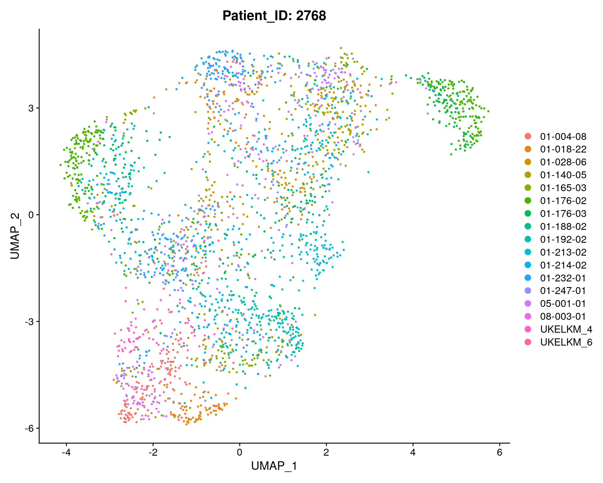
Panel F
fig <- DimPlot(subset, reduction = "umap", group.by = "Group") + ggtitle(paste0("Group: ", length(subset$Group)))

ggsave(here::here("output", DOCNAME, "figure2-panelF.pdf"), fig,
        width = 8, height = 8, scale = 1.2)
ggsave(here::here("output", DOCNAME, "figure2-panelF.png"), fig,
        width = 8, height = 8, scale = 1.2)

fig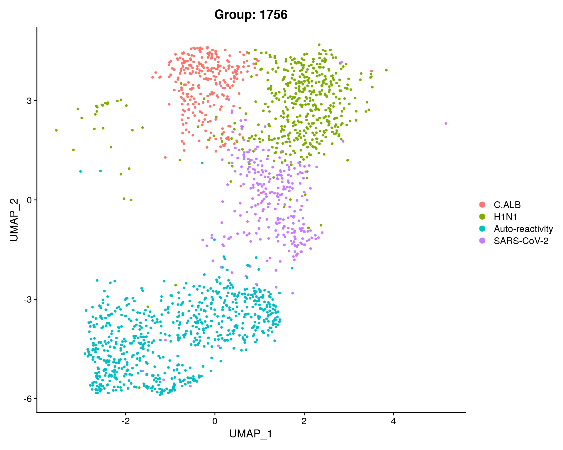
Panel G
fig <- pheatmap(df,
         color = col,
         cluster_rows = FALSE,
         cluster_cols = FALSE,
         show_colnames = FALSE,
         show_rownames = TRUE,
         gaps_col = gap.cells,
         gaps_row = gap.genes,
         fontsize_row = 8 ,
         annotation_col = Annotationcol,
         annotation_colors = annot_colors,
         main = "Heatmap")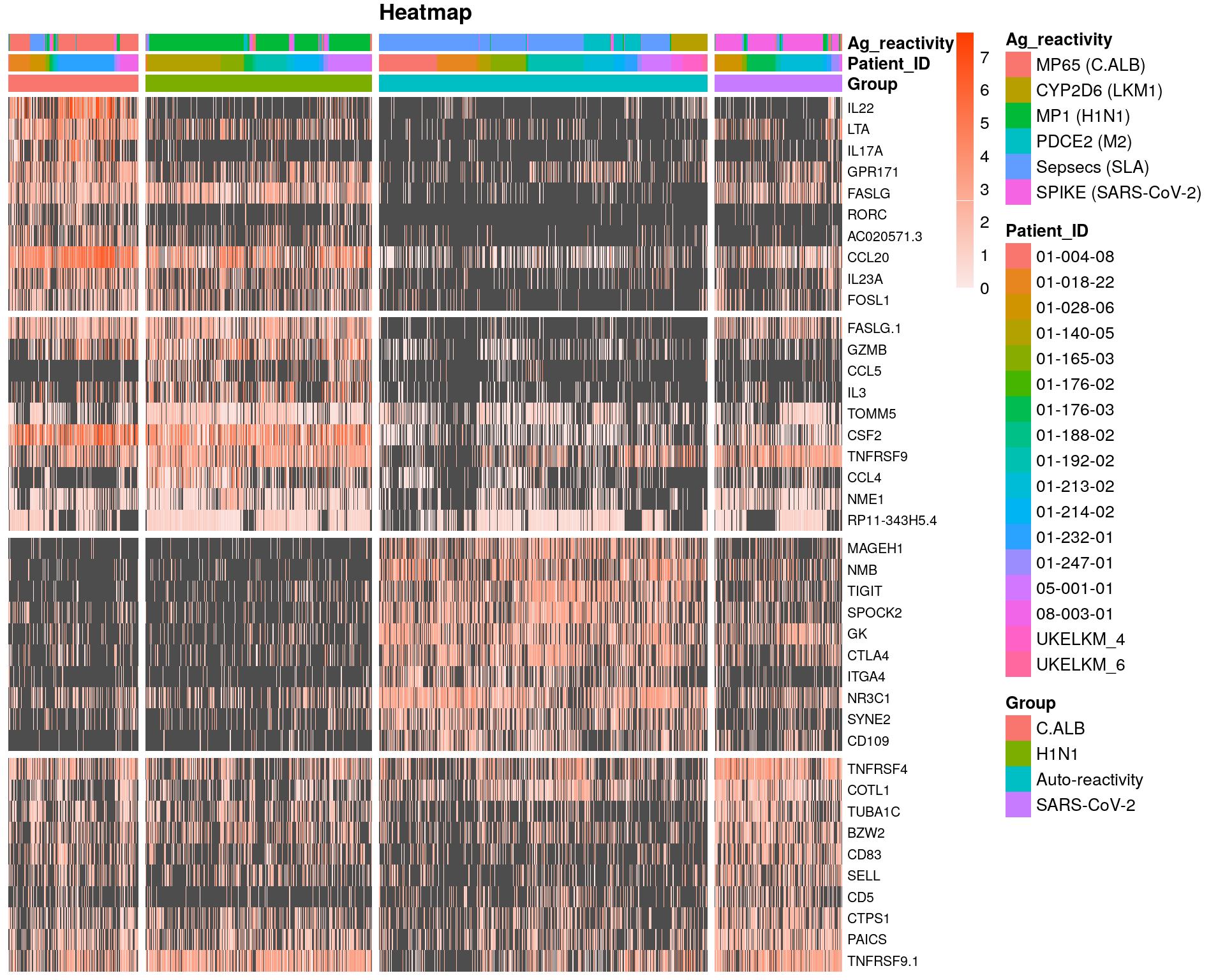
ggsave(here::here("output", DOCNAME, "figure2-panelG.pdf"), fig,
        width = 8, height = 8, scale = 1.2)
ggsave(here::here("output", DOCNAME, "figure2-panelG.png"), fig,
        width = 8, height = 8, scale = 1.2)
Panel H
fig <- DotPlot(subset, features = markers) +
  geom_point(aes(size=pct.exp), shape = 21, colour="black", stroke=0.5) +
  scale_colour_gradient2(low = "grey30",  high = "#FD6839") + # color scale
  guides(size=guide_legend(override.aes=list(shape=21, colour="black", fill="white"))) +
  theme(axis.text.x = element_text(angle = 45, hjust=1))  + coord_flip()

ggsave(here::here("output", DOCNAME, "figure2-panelH.pdf"), fig,
        width = 8, height = 8, scale = 1.2)
ggsave(here::here("output", DOCNAME, "figure2-panelH.png"), fig,
        width = 8, height = 8, scale = 1.2)

fig
Summary
We performed graph based clustering using Seurat and identified 8 clusters, 4 cluster groups of memory CD4 T cells.
Parameters
This table describes parameters used and set in this document.
params <- list(
    list(
        Parameter = "sel_genes",
        Value = length(VariableFeatures(sc_seurat)),
        Description = "Number of selected genes filtered TCR genes based on 4000"
    ),
    list(
        Parameter = "n_pcs",
        Value = n_pcs,
        Description = "Selected number of principal components for clustering"
    ),
    list(
        Parameter = "res",
        Value = resolution,
        Description = "Selected resolution parameter for clustering"
    ),
    list(
        Parameter = "n_clusts",
        Value = n_clusts,
        Description = "Number of clusters produced by selected resolution"
    )
)

params <- jsonlite::toJSON(params, pretty = TRUE)
knitr::kable(jsonlite::fromJSON(params))| Parameter | Value | Description |
|---|---|---|
| sel_genes | 3912 | Number of selected genes filtered TCR genes based on 4000 |
| n_pcs | 40 | Selected number of principal components for clustering |
| res | 0.8 | Selected resolution parameter for clustering |
| n_clusts | 8 | Number of clusters produced by selected resolution |
Output files
saveRDS(sc_seurat, here::here("data/processed/figure2_output_seurat.rds"))
saveRDS(subset, here::here("data/processed/figure2_output_seurat_subset.rds"))
save(metadata_df, file = here::here("data/processed/figure2_output_metadata.RData"))
Session information
devtools::session_info()─ Session info ───────────────────────────────────────────────────────────────
setting value
version R version 4.1.2 (2021-11-01)
os Ubuntu 20.04.3 LTS
system x86_64, linux-gnu
ui X11
language (EN)
collate en_US.UTF-8
ctype en_US.UTF-8
tz Etc/UTC
date 2024-12-24
pandoc 2.14.0.3 @ /usr/lib/rstudio-server/bin/pandoc/ (via rmarkdown)
─ Packages ───────────────────────────────────────────────────────────────────
package * version date (UTC) lib source
abind 1.4-5 2016-07-21 [1] RSPM (R 4.1.0)
assertthat 0.2.1 2019-03-21 [1] RSPM (R 4.1.0)
backports 1.4.1 2021-12-13 [1] RSPM (R 4.1.0)
brio 1.1.3 2021-11-30 [1] RSPM (R 4.1.0)
broom 0.7.12 2022-01-28 [1] RSPM (R 4.1.0)
bslib 0.3.1 2021-10-06 [1] RSPM (R 4.1.0)
cachem 1.0.6 2021-08-19 [1] RSPM (R 4.1.0)
callr 3.7.0 2021-04-20 [1] RSPM (R 4.1.0)
car 3.0-12 2021-11-06 [1] RSPM (R 4.1.0)
carData 3.0-5 2022-01-06 [1] RSPM (R 4.1.0)
cli 3.6.1 2023-03-23 [1] RSPM (R 4.1.0)
cluster 2.1.2 2021-04-17 [2] CRAN (R 4.1.2)
codetools 0.2-18 2020-11-04 [2] CRAN (R 4.1.2)
colorspace 2.0-3 2022-02-21 [1] RSPM (R 4.1.0)
cowplot * 1.1.1 2020-12-30 [1] RSPM (R 4.1.0)
crayon 1.5.0 2022-02-14 [1] RSPM (R 4.1.0)
data.table 1.14.2 2021-09-27 [1] RSPM (R 4.1.0)
DBI 1.1.2 2021-12-20 [1] RSPM (R 4.1.0)
deldir 1.0-6 2021-10-23 [1] RSPM (R 4.1.0)
desc 1.4.1 2022-03-06 [1] RSPM (R 4.1.0)
devtools 2.4.3 2021-11-30 [1] RSPM (R 4.1.0)
digest 0.6.29 2021-12-01 [1] RSPM (R 4.1.0)
dplyr 1.0.8 2022-02-08 [1] RSPM (R 4.1.0)
DT * 0.22 2022-03-28 [1] RSPM (R 4.1.0)
ellipsis 0.3.2 2021-04-29 [1] RSPM (R 4.1.0)
evaluate 0.15 2022-02-18 [1] RSPM (R 4.1.0)
fansi 1.0.2 2022-01-14 [1] RSPM (R 4.1.0)
fastmap 1.1.0 2021-01-25 [1] RSPM (R 4.1.0)
fitdistrplus 1.1-6 2021-09-28 [1] RSPM (R 4.1.0)
fs 1.5.2 2021-12-08 [1] RSPM (R 4.1.0)
future 1.23.0 2021-10-31 [1] RSPM (R 4.1.0)
future.apply 1.8.1 2021-08-10 [1] RSPM (R 4.1.0)
generics 0.1.2 2022-01-31 [1] RSPM (R 4.1.0)
ggplot2 * 3.4.4 2023-10-12 [1] RSPM (R 4.1.0)
ggpubr * 0.4.0 2020-06-27 [1] RSPM (R 4.1.0)
ggrepel 0.9.1 2021-01-15 [1] RSPM (R 4.1.0)
ggridges 0.5.3 2021-01-08 [1] RSPM (R 4.1.0)
ggsignif 0.6.3 2021-09-09 [1] RSPM (R 4.1.0)
git2r 0.33.0 2023-11-26 [1] RSPM (R 4.1.0)
globals 0.14.0 2020-11-22 [1] RSPM (R 4.1.0)
glue 1.6.2 2022-02-24 [1] RSPM (R 4.1.0)
goftest 1.2-3 2021-10-07 [1] RSPM (R 4.1.0)
gridExtra 2.3 2017-09-09 [1] RSPM (R 4.1.0)
gtable 0.3.0 2019-03-25 [1] RSPM (R 4.1.0)
here 1.0.1 2020-12-13 [1] RSPM (R 4.1.0)
htmltools 0.5.2 2021-08-25 [1] RSPM (R 4.1.0)
htmlwidgets 1.5.4 2021-09-08 [1] RSPM (R 4.1.0)
httpuv 1.6.5 2022-01-05 [1] RSPM (R 4.1.0)
httr 1.4.2 2020-07-20 [1] RSPM (R 4.1.0)
ica 1.0-2 2018-05-24 [1] RSPM (R 4.1.0)
igraph 1.5.1 2023-08-10 [1] RSPM (R 4.1.0)
irlba 2.3.5 2021-12-06 [1] RSPM (R 4.1.0)
jquerylib 0.1.4 2021-04-26 [1] RSPM (R 4.1.0)
jsonlite 1.8.0 2022-02-22 [1] RSPM (R 4.1.0)
KernSmooth 2.23-20 2021-05-03 [2] CRAN (R 4.1.2)
knitr * 1.37 2021-12-16 [1] RSPM (R 4.1.0)
later 1.3.0 2021-08-18 [1] RSPM (R 4.1.0)
lattice 0.20-45 2021-09-22 [2] CRAN (R 4.1.2)
lazyeval 0.2.2 2019-03-15 [1] RSPM (R 4.1.0)
leiden 0.3.9 2021-07-27 [1] RSPM (R 4.1.0)
lifecycle 1.0.3 2022-10-07 [1] RSPM (R 4.1.0)
listenv 0.8.0 2019-12-05 [1] RSPM (R 4.1.0)
lmtest 0.9-39 2021-11-07 [1] RSPM (R 4.1.0)
magrittr 2.0.2 2022-01-26 [1] RSPM (R 4.1.0)
MASS 7.3-54 2021-05-03 [2] CRAN (R 4.1.2)
Matrix 1.3-4 2021-06-01 [2] CRAN (R 4.1.2)
matrixStats 0.61.0 2021-09-17 [1] RSPM (R 4.1.0)
memoise 2.0.1 2021-11-26 [1] RSPM (R 4.1.0)
mgcv 1.8-38 2021-10-06 [2] CRAN (R 4.1.2)
mime 0.12 2021-09-28 [1] RSPM (R 4.1.0)
miniUI 0.1.1.1 2018-05-18 [1] RSPM (R 4.1.0)
munsell 0.5.0 2018-06-12 [1] RSPM (R 4.1.0)
nlme 3.1-153 2021-09-07 [2] CRAN (R 4.1.2)
parallelly 1.30.0 2021-12-17 [1] RSPM (R 4.1.0)
patchwork 1.1.1 2020-12-17 [1] RSPM (R 4.1.0)
pbapply 1.5-0 2021-09-16 [1] RSPM (R 4.1.0)
pheatmap * 1.0.12 2019-01-04 [1] RSPM (R 4.1.0)
pillar 1.7.0 2022-02-01 [1] RSPM (R 4.1.0)
pkgbuild 1.3.1 2021-12-20 [1] RSPM (R 4.1.0)
pkgconfig 2.0.3 2019-09-22 [1] RSPM (R 4.1.0)
pkgload 1.2.4 2021-11-30 [1] RSPM (R 4.1.0)
plotly 4.10.0 2021-10-09 [1] RSPM (R 4.1.0)
plyr 1.8.6 2020-03-03 [1] RSPM (R 4.1.0)
png 0.1-7 2013-12-03 [1] RSPM (R 4.1.0)
polyclip 1.10-0 2019-03-14 [1] RSPM (R 4.1.0)
prettyunits 1.1.1 2020-01-24 [1] RSPM (R 4.1.0)
processx 3.5.2 2021-04-30 [1] RSPM (R 4.1.0)
promises 1.2.0.1 2021-02-11 [1] RSPM (R 4.1.0)
ps 1.6.0 2021-02-28 [1] RSPM (R 4.1.0)
purrr 0.3.4 2020-04-17 [1] RSPM (R 4.1.0)
R6 2.5.1 2021-08-19 [1] RSPM (R 4.1.0)
RANN 2.6.1 2019-01-08 [1] RSPM (R 4.1.0)
RColorBrewer 1.1-2 2014-12-07 [1] RSPM (R 4.1.0)
Rcpp 1.0.8 2022-01-13 [1] RSPM (R 4.1.0)
RcppAnnoy 0.0.19 2021-07-30 [1] RSPM (R 4.1.0)
remotes 2.4.2 2021-11-30 [1] RSPM (R 4.1.0)
reshape2 1.4.4 2020-04-09 [1] RSPM (R 4.1.0)
reticulate 1.23 2022-01-14 [1] RSPM (R 4.1.0)
rlang 1.1.1 2023-04-28 [1] RSPM (R 4.1.0)
rmarkdown 2.11 2021-09-14 [1] RSPM (R 4.1.0)
ROCR 1.0-11 2020-05-02 [1] RSPM (R 4.1.0)
rpart 4.1-15 2019-04-12 [2] CRAN (R 4.1.2)
rprojroot 2.0.2 2020-11-15 [1] RSPM (R 4.1.0)
rstatix 0.7.0 2021-02-13 [1] RSPM (R 4.1.0)
rstudioapi 0.13 2020-11-12 [1] RSPM (R 4.1.0)
Rtsne 0.15 2018-11-10 [1] RSPM (R 4.1.0)
sass 0.4.0 2021-05-12 [1] RSPM (R 4.1.0)
scales 1.2.1 2022-08-20 [1] RSPM (R 4.1.0)
scattermore 0.7 2020-11-24 [1] RSPM (R 4.1.0)
sctransform 0.3.3 2022-01-13 [1] RSPM (R 4.1.0)
sessioninfo 1.2.2 2021-12-06 [1] RSPM (R 4.1.0)
Seurat * 4.1.0 2022-01-14 [1] RSPM (R 4.1.0)
SeuratObject * 4.0.4 2021-11-23 [1] RSPM (R 4.1.0)
shiny 1.7.1 2021-10-02 [1] RSPM (R 4.1.0)
spatstat.core 2.3-2 2021-11-26 [1] RSPM (R 4.1.0)
spatstat.data 2.1-2 2021-12-17 [1] RSPM (R 4.1.0)
spatstat.geom 2.4-0 2022-03-29 [1] RSPM (R 4.1.0)
spatstat.sparse 2.1-0 2021-12-17 [1] RSPM (R 4.1.0)
spatstat.utils 2.3-0 2021-12-12 [1] RSPM (R 4.1.0)
stringi 1.7.6 2021-11-29 [1] RSPM (R 4.1.0)
stringr 1.4.0 2019-02-10 [1] RSPM (R 4.1.0)
survival 3.2-13 2021-08-24 [2] CRAN (R 4.1.2)
tensor 1.5 2012-05-05 [1] RSPM (R 4.1.0)
testthat 3.1.2 2022-01-20 [1] RSPM (R 4.1.0)
tibble 3.1.8 2022-07-22 [1] RSPM (R 4.1.0)
tidyr 1.2.0 2022-02-01 [1] RSPM (R 4.1.0)
tidyselect 1.1.2 2022-02-21 [1] RSPM (R 4.1.0)
usethis 2.1.5 2021-12-09 [1] RSPM (R 4.1.0)
utf8 1.2.2 2021-07-24 [1] RSPM (R 4.1.0)
uwot 0.1.11 2021-12-02 [1] RSPM (R 4.1.0)
vctrs 0.6.4 2023-10-12 [1] RSPM (R 4.1.0)
viridisLite 0.4.0 2021-04-13 [1] RSPM (R 4.1.0)
withr 2.5.0 2022-03-03 [1] RSPM (R 4.1.0)
workflowr 1.7.1 2023-08-23 [1] RSPM (R 4.1.0)
xfun 0.30 2022-03-02 [1] RSPM (R 4.1.0)
xtable 1.8-4 2019-04-21 [1] RSPM (R 4.1.0)
yaml 2.3.5 2022-02-21 [1] RSPM (R 4.1.0)
zoo 1.8-9 2021-03-09 [1] RSPM (R 4.1.0)
[1] /usr/local/lib/R/site-library
[2] /usr/local/lib/R/library
──────────────────────────────────────────────────────────────────────────────
sessionInfo()R version 4.1.2 (2021-11-01)
Platform: x86_64-pc-linux-gnu (64-bit)
Running under: Ubuntu 20.04.3 LTS
Matrix products: default
BLAS/LAPACK: /usr/lib/x86_64-linux-gnu/openblas-pthread/libopenblasp-r0.3.8.so
locale:
[1] LC_CTYPE=en_US.UTF-8 LC_NUMERIC=C LC_TIME=en_US.UTF-8 LC_COLLATE=en_US.UTF-8 LC_MONETARY=en_US.UTF-8 LC_MESSAGES=en_US.UTF-8 LC_PAPER=en_US.UTF-8 LC_NAME=C LC_ADDRESS=C
[10] LC_TELEPHONE=C LC_MEASUREMENT=en_US.UTF-8 LC_IDENTIFICATION=C
attached base packages:
[1] stats graphics grDevices utils datasets methods base
other attached packages:
[1] pheatmap_1.0.12 forcats_0.5.1 stringr_1.4.0 purrr_0.3.4 readr_2.1.1 tidyr_1.2.0 tibble_3.1.8 tidyverse_1.3.1 jsonlite_1.8.0 glue_1.6.2 dplyr_1.0.8 DT_0.22
[13] readxl_1.3.1 knitr_1.37 cowplot_1.1.1 ggpubr_0.4.0 ggplot2_3.4.4 SeuratObject_4.0.4 Seurat_4.1.0
loaded via a namespace (and not attached):
[1] utf8_1.2.2 reticulate_1.23 tidyselect_1.1.2 htmlwidgets_1.5.4 grid_4.1.2 Rtsne_0.15 devtools_2.4.3 munsell_0.5.0 codetools_0.2-18 ragg_1.2.2 ica_1.0-2
[12] future_1.23.0 miniUI_0.1.1.1 withr_2.5.0 colorspace_2.0-3 highr_0.9 rstudioapi_0.13 ROCR_1.0-11 ggsignif_0.6.3 tensor_1.5 listenv_0.8.0 labeling_0.4.2
[23] git2r_0.33.0 polyclip_1.10-0 bit64_4.0.5 farver_2.1.0 rprojroot_2.0.2 parallelly_1.30.0 vctrs_0.6.4 generics_0.1.2 xfun_0.30 R6_2.5.1 spatstat.utils_2.3-0
[34] cachem_1.0.6 assertthat_0.2.1 promises_1.2.0.1 scales_1.2.1 vroom_1.5.7 gtable_0.3.0 globals_0.14.0 processx_3.5.2 goftest_1.2-3 workflowr_1.7.1 rlang_1.1.1
[45] systemfonts_1.0.4 splines_4.1.2 rstatix_0.7.0 lazyeval_0.2.2 spatstat.geom_2.4-0 broom_0.7.12 yaml_2.3.5 reshape2_1.4.4 abind_1.4-5 modelr_0.1.8 crosstalk_1.2.0
[56] backports_1.4.1 httpuv_1.6.5 tools_4.1.2 usethis_2.1.5 ellipsis_0.3.2 spatstat.core_2.3-2 jquerylib_0.1.4 RColorBrewer_1.1-2 sessioninfo_1.2.2 ggridges_0.5.3 Rcpp_1.0.8
[67] plyr_1.8.6 ps_1.6.0 prettyunits_1.1.1 rpart_4.1-15 deldir_1.0-6 pbapply_1.5-0 zoo_1.8-9 haven_2.4.3 ggrepel_0.9.1 cluster_2.1.2 fs_1.5.2
[78] here_1.0.1 magrittr_2.0.2 data.table_1.14.2 RSpectra_0.16-0 scattermore_0.7 lmtest_0.9-39 reprex_2.0.1 RANN_2.6.1 fitdistrplus_1.1-6 matrixStats_0.61.0 pkgload_1.2.4
[89] hms_1.1.1 patchwork_1.1.1 mime_0.12 evaluate_0.15 xtable_1.8-4 gridExtra_2.3 testthat_3.1.2 compiler_4.1.2 KernSmooth_2.23-20 crayon_1.5.0 htmltools_0.5.2
[100] mgcv_1.8-38 later_1.3.0 tzdb_0.2.0 lubridate_1.8.0 DBI_1.1.2 dbplyr_2.1.1 MASS_7.3-54 Matrix_1.3-4 car_3.0-12 brio_1.1.3 cli_3.6.1
[111] parallel_4.1.2 igraph_1.5.1 pkgconfig_2.0.3 plotly_4.10.0 spatstat.sparse_2.1-0 xml2_1.3.3 bslib_0.3.1 rvest_1.0.2 callr_3.7.0 digest_0.6.29 sctransform_0.3.3
[122] RcppAnnoy_0.0.19 spatstat.data_2.1-2 rmarkdown_2.11 cellranger_1.1.0 leiden_0.3.9 uwot_0.1.11 shiny_1.7.1 lifecycle_1.0.3 nlme_3.1-153 carData_3.0-5 desc_1.4.1
[133] viridisLite_0.4.0 limma_3.50.1 fansi_1.0.2 pillar_1.7.0 lattice_0.20-45 fastmap_1.1.0 httr_1.4.2 pkgbuild_1.3.1 survival_3.2-13 remotes_2.4.2 png_0.1-7
[144] bit_4.0.4 stringi_1.7.6 sass_0.4.0 textshaping_0.3.6 memoise_2.0.1 irlba_2.3.5 future.apply_1.8.1